#62 Optical coherence tomography-IV 光學相干斷層掃描_下

I am so happy that we finally reach the end of this series. Today we are going to do a computer simulation experiment using MATLAB to demonstrate the key concepts of OCT, including TDOCT & FDOCT.
很高興終於來到最後一集了><!!今天我們要用MATLAB來做個OCT的模擬實驗，我們會先做TDOCT，然後再做FDOCT，並演示一些OCT的重要觀念。

%% Basic Settings
k0 = 12E6; %central wave number, green light
delk = 3E6; %wave number spread
S_k = @(k) 1./(delk*sqrt(pi)).*exp(-((k-k0)/delk).^2); %power spectrum of light source
figure
h = ezplot(S_k, [4E6, 20E6]);
title('low coherence light source spectrum', 'Fontsize', 12, 'Fontweight', 'bold'); xlabel('wave number(m^{-1})', 'Fontsize', 12, 'Fontweight', 'bold'); ylabel('Relative intensity', 'Fontsize', 12, 'Fontweight', 'bold'); set(gca, 'Fontsize', 12, 'Fontweight', 'bold');
set(h,'Linewidth',2);
print('low coherence light source spectrum','-dpng');
zs1 = 0.024000; rs1 = 0.00025;%normal eye AP length
zs2 = 0.024030; rs2 = 0.00010;
zs3 = 0.024090; rs3 = 0.00015;
zs4 = 0.024150; rs4 = 0.00005;
zs5 = 0.024200; rs5 = 0.00020;
zs6 = 0.024310; rs6 = 0.00010;
zs7 = 0.024350; rs7 = 0.00030;%artificial retina layers settings
zs8 = 0.025000; rs8 = 0.99100;%sclera
rR = 1; % reflectivity of reference reflector

We first setup the parameters of the system. We simulate a retina with only 7 layers (there are in fact 10 layers) for simplification. The 8th layer is sclera with significantly larger reflection rate, which allows us to observe the effect of having a layer with high reflection rate. One line in the above code could show the spectrum of the light we are using. Let's see how it looks like:
第一段我們先來建設一些基本設置，我們想要模擬一個視網膜，為了簡化，我們只放7層結構，第八層是鞏膜，有比其他層明顯較高的反射率，我們可以順便看看這會有甚麼影響。其中有一行print出我們使用的光源的光譜，我們來看一下長甚麼樣子：

It looks like our light source have a broad spectrum and low coherence. I bet it could serve well. Now let's start our experiment from TDOCT.
嗯，光譜散得很開，看起來是一個low cohenece的光源，相信他可以勝任愉快。我們接下來就要進行模擬實驗了，我們先從簡單的TDOCT開始。

%% normal setting demonstration
E_R = @(zr, k) sqrt(S_k(k))/2*rR.*exp(1i*2*k*zr);
E_s = @(k) sqrt(S_k(k))/2.*(rs1*exp(1i*2*k*zs1) +rs2*exp(1i*2*k*zs2) + rs3*exp(1i*2*k*zs3) + rs4*exp(1i*2*k*zs4) + rs5*exp(1i*2*k*zs5) + rs6*exp(1i*2*k*zs6) + rs7*exp(1i*2*k*zs7) + rs8*exp(1i*2*k*zs8));
%TDOCT
zr_range = 0.023500:0.000001:0.024500; %scanning distance range, does not include sclera
E_R_range = @(k) E_R(zr_range, k);
I_D_TDOCT = @(k) (abs(E_R_range(k) + E_s(k))).^2;
I_D_zr = integral(I_D_TDOCT, 4E6, 20E6, 'ArrayValued', true);
figure, plot(zr_range, I_D_zr, 'Linewidth',2); xlim([0.023500, 0.024500]);
title('TDOCT result, low coherence light source', 'Fontsize', 12, 'Fontweight', 'bold');xlabel('z_R(m)', 'Fontsize', 12, 'Fontweight', 'bold');ylabel('I_D(z_R)', 'Fontsize', 12, 'Fontweight', 'bold');set(gca, 'Fontsize', 12, 'Fontweight', 'bold');%plot TDOCT result
print('TDOCT low coherence light source ','-dpng');

We first write down the electric field coming from reference optical path and sample optical path, then adjust the scanning depth of reference optical path, and finally sum the energy of all light with different wavelengths. By doing so, we leave only the cross correlation term retaining its dependency on the reference optical path length. Let's see our result:
我們先寫出了參考光徑的反射光與樣本路徑的反射光的電場形式之後，我們調整我們要掃描的參考光徑長，然後在每個長度之下，把不同波長的光能全部加總。藉由這個方式，原本測得的電流讀值有三個terms，現在就只剩下cross correlation terms還保有對參考光徑長的dependency，其他兩項都變成常數，我們來看看最後面print出來的結果：

It looks really great, right? We then have to check the peak location by labeling them...
看起來真的很不錯對吧？我們再來要核對一下出現peak的位置是不是就是我們要的位置，所以我們用data cursor把peak的位置標一標：

They perfectly match our initial settings! However, it should be noted that we did not detect the sclera because we did not adjust our reference optical path till 0.025000 m. This is the main problem of TDOCT. The accuracy and the range of reference optical path length directly determine what you will get. That's all for the TDOCT. Let's move on to FDOCT.
和我們前面第一段設定的位置一模一樣呢！不過要注意的是，因為我們掃描的深度沒有到sclera的地方，所以sclera的反射波不會被讀出來。這也說明了TDOCT的缺點──你想要掃到多深，就必須調整參考光徑到多長。你想要量得多精細，參考光徑調整路徑長的解析度就要有多高！！TDOCT的部分結束，我們再來看FDOCT的部分。

%FDOCT-1
zr1 = 0.023500; %an appropriate zr choice
E_R_k = @(k) E_R(zr1, k);
I_D_FDOCT1 = @(k) abs(E_s(k)+E_R_k(k)).^2;
k_range = 8E6:1E3:14E6;
delX = pi/(2*(14E6-8E6));
x_range = 0:delX:delX*(length(k_range)-1);
I_D_k1 = I_D_FDOCT1(k_range);
i_D_z1 = dct(I_D_k1); %discrete cosine transform
%figure, plot(x_range+zr1, i_D_z1);
figure, plot(x_range+zr1, log(abs(i_D_z1)),  'Linewidth',2);%to illustrate the peak
title('FDOCT result, low coherence, correct z_R choice', 'Fontsize', 12, 'Fontweight', 'bold');xlabel('z_s(m)', 'Fontsize', 12, 'Fontweight', 'bold');ylabel('i_D(z_s)', 'Fontsize', 12, 'Fontweight', 'bold');set(gca, 'Fontsize', 12, 'Fontweight', 'bold');
print('FDOCT result low coherence correct zR','-dpng');

We will play the FDOCT twice. One with appropriate reference optical length while the other inappropriate. In FDOCT, we record the interference of different wavelength, transform it into z-domain with Fourier transform, and finally check the location of the peak. In the following figure we have already add back the reference optical path length to our peak locations.
我們FDOCT會做兩個，一個先選取適當的參考光徑長度，另一個選取不適當的參考光徑長度。我們把不同波長的干涉結果記錄下來，然後傅立葉轉換到z-domain，來看看peak的位置在哪裡。注意我們已經把參考光徑的長度加回去了，原本的結果讀出來的數值會是反射層位置與參考光徑長的長度差。

The FDOCT results look great, too. But we still have to check the location of peaks......
看起來也很不錯呢，不過我們來看看這些peak的位置正不正確：

These peaks look okay. What about the other ones?
左邊這些peak大致上都還好。那右邊呢？

You must have noticed some false peaks in our results. How could they even exist??? Actually this is a trap set by me. I hope everyone could remind himself/herself of the short-coming of FDOCT?? The locations of these false peaks are actually predictable. Please carefully figure it out by yourself.
和最一開始的設定值比較一下，我們可以發現出現了好幾個假peak耶！？這是為甚麼呢？？這其實是小編故意設下的，專屬於FDOCT的陷阱喔~~~。請讀者好好思考思考，這些假peak的位置都是可以預期的，如果想不通，把前一集(http://biophys3min.blogspot.tw/2016/07/61.html)好好拿出來讀一讀，再想不通的話歡迎在網誌或粉絲專頁上留言喔。

Now let's see what would happen if we initially set an inappropriate reference optical path lengh.
我們再來看看如果我們把參考光徑設定為一個不恰當的長度會發生甚麼事情：

%FDOCT-2
zr2 = 0.024500; %an inappropriate zr choice
E_R_k = @(k) E_R(zr2, k);
I_D_FDOCT2 = @(k) abs(E_s(k)+E_R_k(k)).^2;
k_range = 8E6:1E3:14E6;
I_D_k2 = I_D_FDOCT2(k_range);
i_D_z2 = dct(I_D_k2); %discrete cosine transform
%figure, plot(x_range+zr2, i_D_z2);
figure, plot(x_range+zr2, log(abs(i_D_z2)),  'Linewidth',2);%to illustrate the peak
title('FDOCT result, low coherence, incorrect z_R choice', 'Fontsize', 12, 'Fontweight', 'bold');xlabel('z_s(m)', 'Fontsize', 12, 'Fontweight', 'bold');ylabel('i_D(z_s)', 'Fontsize', 12, 'Fontweight', 'bold');set(gca, 'Fontsize', 12, 'Fontweight', 'bold');
print('FDOCT result low coherence incorrect zR','-dpng');

Let's see our results......
廢話不多說直接看結果：

I guess it looks bad enough already. Please remember to check the appropriateness of the reference optical path length.
應該不用我說也知道這看起來不是很好處理。所以參考光徑要選取適當喔！

And finally let's see what would happen if we use a highly coherent light source such as laser for our OCT experiment:
我們最後來看看，如果用高度相干光源來做實驗會發生甚麼事情：

%% coherent light source
k0 = 12E6; %central wave number, green light
delk = 1E4; %wave number spread
S_k = @(k) 1./(delk*sqrt(pi)).*exp(-((k-k0)/delk).^2);
figure
h= ezplot(S_k, [4E6, 20E6]); ylim([0, 6E-6]);
set(h,'Linewidth',2);
title('high coherence light source spectrum', 'Fontsize', 12, 'Fontweight', 'bold'); xlabel('wave number(m^{-1})', 'Fontsize', 12, 'Fontweight', 'bold'); ylabel('Relative intensity', 'Fontsize', 12, 'Fontweight', 'bold'); set(gca, 'Fontsize', 12, 'Fontweight', 'bold');
print('high coherence light source spectrum','-dpng');
E_R = @(zr, k) sqrt(S_k(k))/2*rR.*exp(1i*2*k*zr);
E_s = @(k) sqrt(S_k(k))/2.*(rs1*exp(1i*2*k*zs1) +rs2*exp(1i*2*k*zs2) + rs3*exp(1i*2*k*zs3) + rs4*exp(1i*2*k*zs4) + rs5*exp(1i*2*k*zs5) + rs6*exp(1i*2*k*zs6) + rs7*exp(1i*2*k*zs7) + rs8*exp(1i*2*k*zs8));

The spectrum of our light source looks like this:
來看看跑出來的光譜：

It's highly coherent and looks sexy. However, we will soon realize that using a laser for OCT is definitely the most foolish idea that you could ever come up with.
WOW還真是個高度相干的光源呢真好，不過我們很快就會看到，用高度相干光源來做OCT絕對會是一場史無前例的大災難，是人生中最錯誤的選擇沒有之一。

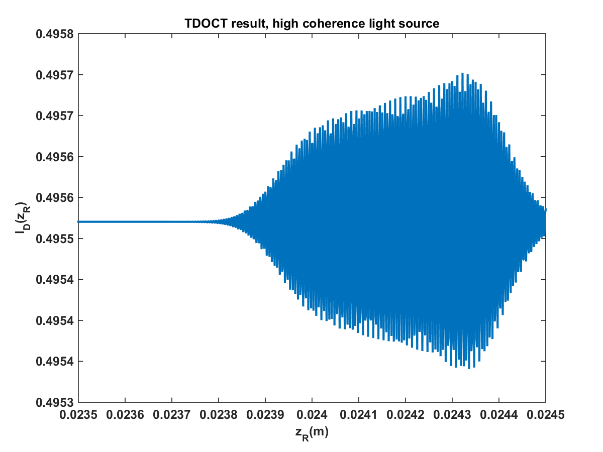
Let's see the TDOCT results using a laser:
來看看用高度相干光源做TDOCT的結果：

%TDOCT
zr_range = 0.023500:0.000001:0.024500; %scanning distance range, does not include sclera
E_R_range = @(k) E_R(zr_range, k);
I_D_TDOCT = @(k) (abs(E_R_range(k) + E_s(k))).^2;
I_D_zr = integral(I_D_TDOCT, 4E6, 20E6, 'ArrayValued', true);
figure, plot(zr_range, I_D_zr, 'Linewidth',2); xlim([0.023500, 0.024500]);
title('TDOCT result, high coherence light source', 'Fontsize', 12, 'Fontweight', 'bold');xlabel('z_R(m)', 'Fontsize', 12, 'Fontweight', 'bold');ylabel('I_D(z_R)', 'Fontsize', 12, 'Fontweight', 'bold');set(gca, 'Fontsize', 12, 'Fontweight', 'bold');%plot TDOCT result
print('TDOCT high coherence light source ','-dpng');

I guess it's needless to explain anything now: it just looks terrible. Let's then see how would FDOCT looks like using a laser:
拿去和前面的TDOCT實驗結果對照一下，如果你是菸酒生應該會很想去撞牆吧！這樣各位懂了嗎~~？我們再來看看FDOCT的結果：

%FDOCT
zr1 = 0.023500; %an appropriate zr choice
E_R_k = @(k) E_R(zr1, k);
I_D_FDOCT1 = @(k) abs(E_s(k)+E_R_k(k)).^2;
k_range = 8E6:1E3:14E6;
delX = pi/(2*(14E6-8E6));
x_range = 0:delX:delX*(length(k_range)-1);
I_D_k1 = I_D_FDOCT1(k_range);
i_D_z1 = dct(I_D_k1); %discrete cosine transform
figure, plot(x_range+zr1, log(abs(i_D_z1)), 'Linewidth',2);%to illustrate the peak
title('FDOCT result, high coherence', 'Fontsize', 12, 'Fontweight', 'bold');xlabel('z_s(m)', 'Fontsize', 12, 'Fontweight', 'bold');ylabel('i_D(z_s)', 'Fontsize', 12, 'Fontweight', 'bold');set(gca, 'Fontsize', 12, 'Fontweight', 'bold');
print('FDOCT result high coherence','-dpng');

As disastrous as the previous one.
又是一個慘不忍睹，還以為是倒著看麥X勞呢。

We hope that after these 4 episodes, all of you could understand the basic principles of OCT!
希望經過這四集的介紹，各位都能更明白OCT的原理喔！！