- Get link
- X
- Other Apps
Hello. Today we will use MATLAB program for simulation of gradient sensing by slime mold. In our previous episode we have write down explicitly the estimated concentration gradient in z direction by monitoring the position of inward particle flow and summing their cosine. That is
哈囉~,前面幾集我們已經討論過黏菌可以利用maximum likelihood estimation,紀錄粒子流入的位置,回推背景梯度。今天我們要用MATLAB來模擬這個情形,然後看看他的效果如何。上一集我們有提到最後利用MLE算得的z方向梯度是:

In the first part of our code we simply set the location of our slime mold cell and the speed of our nutrient particle. The diffusion constant D is calculated by knowing in 3D world, <r^2>=6DT.
在第一部分的程式中我們就只是把一些基本參數設定一下,包括黏菌細胞的大小位置,還有粒子的速度。擴散係數D的寫法是利用了<r^2>=6DT的關係式。

And we could start our experiment:
然後就開始實驗

}{\partial&space;x}=-\sigma/2\\&space;\sigma=\frac{1}{\Delta&space;TW^2}\\&space;c(x=L)=0\\&space;c(x=-L)=0 "\\ D\frac{\partial^2 c}{\partial x^2}=0\\ D\frac{\partial c(x=0)}{\partial x}=-\sigma/2\\ \sigma=\frac{1}{\Delta TW^2}\\ c(x=L)=0\\ c(x=-L)=0")
哈囉~,前面幾集我們已經討論過黏菌可以利用maximum likelihood estimation,紀錄粒子流入的位置,回推背景梯度。今天我們要用MATLAB來模擬這個情形,然後看看他的效果如何。上一集我們有提到最後利用MLE算得的z方向梯度是:
So let's see how efficient and accurate it is.
今天就來看看他的效果吧!
今天就來看看他的效果吧!
Our MATLAB script
%% Basic setting
tic; clear; clc;
r_Dicty = 0;
location_Dicty = [10,0, 0];
x_source = 0;
width_source = 15;
x_Boundary = 20;
speed = 0.1;
D = speed^2/6;
t = 1;
tRun = 40000;
Detected_List = nan(tRun, 3);
x_particle_all = nan(tRun, 3);
v_particle_all = nan(tRun, 3);
location_Dicty_rpt = repmat(location_Dicty, tRun, 1);
In the first part of our code we simply set the location of our slime mold cell and the speed of our nutrient particle. The diffusion constant D is calculated by knowing in 3D world, <r^2>=6DT.
在第一部分的程式中我們就只是把一些基本參數設定一下,包括黏菌細胞的大小位置,還有粒子的速度。擴散係數D的寫法是利用了<r^2>=6DT的關係式。
%% get into steady state before our experiment
while t<=tRun
    theta = rand(1,1)*pi; phi = rand(1,1)*2*pi;
    y_source = width_source*(rand(1,1)-0.5);
    z_source = width_source*(rand(1,1)-0.5);
    x_particle_all(t, :) = [x_source, y_source, z_source];
    v_particle_all(t, :) = [cos(phi)*sin(theta), sin(phi)*sin(theta), cos(theta)];
    %move
    x_particle_all = x_particle_all + v_particle_all*speed;
    %check collapse boundary
    a = x_particle_all(:,1)<0 -="" a="" b="x_particle_all(:,1)" v_particle_all="" x_particle_all=""> x_Boundary;
    x_particle_all(b,:) = nan;
    v_particle_all(b,:) = nan;
    c = x_particle_all(:,2) > 0.5*width_source;
    x_particle_all(c,2) = x_particle_all(c,2) - width_source;
    d = x_particle_all(:,2) < -0.5*width_source;
    x_particle_all(d,2) = x_particle_all(d,2) + width_source;
    e = x_particle_all(:,3) > 0.5*width_source;
    x_particle_all(e,3) = x_particle_all(e,3) - width_source;
    f = x_particle_all(:,3) < -0.5*width_source;
    x_particle_all(f,3) = x_particle_all(f,3) + width_source;
    %check collapse detector
    dist_all = (sum((x_particle_all - location_Dicty_rpt).^2, 2)).^0.5;
    e = dist_all <= r_Dicty;
    Detected_List(e,:) = x_particle_all(e,:);
    x_particle_all(e,:) = nan; v_particle_all(e,:) = nan;
    %change direction
    b = ~isnan(v_particle_all);
    c = b(:,1)&b(:,2);
    d = 2*pi*rand(tRun,1); e = pi*rand(tRun,1);
    v_particle_all = [sin(e).*cos(d), sin(e).*sin(d), cos(e)];
    v_particle_all(~c,:) = nan;
    %next round
    t = t + 1;
    %display(t);
end
Because our experimental environment is a 15x15x20 hexahedral, which is quite large and is able to accommodate lots of particles, so before our experiment we must have our particle diffusion get into steady state. The above code could also be written in object-oriented coding. However, it would be much much more efficient in MATLAB if you could express everything you need to do in matrix form. The particles are generated in the left boundary and disappear if they collapse the right boundary. Let's see the result of above code:
因為我們的實驗環境是15x15x20,算是蠻大的而且可以容納非常多粒子,所以我們必須先讓實驗環境達到穩定狀態之後才可以把細胞放進去。上面的程式可以用物件導向程式設計完成,但是因為我們是用MATLAB,如果你可以用矩陣表示就盡量用矩陣,會快非常非常多。在上面的程式中粒子從左邊的邊界製造,一碰到右側邊界就消滅。上面那一串RUN出來的結果會長這樣:
因為我們的實驗環境是15x15x20,算是蠻大的而且可以容納非常多粒子,所以我們必須先讓實驗環境達到穩定狀態之後才可以把細胞放進去。上面的程式可以用物件導向程式設計完成,但是因為我們是用MATLAB,如果你可以用矩陣表示就盡量用矩陣,會快非常非常多。在上面的程式中粒子從左邊的邊界製造,一碰到右側邊界就消滅。上面那一串RUN出來的結果會長這樣:
Hmm, it looks like it is now in steady state. (Of course there are some ways to check if it is in steady state already. How will you do?) So now let's place our slime mold in the center.
如我們預期的產生一個美美的梯度,看起來應該也達到穩定狀態了(當然其實有方式可以檢查系統到底有沒有達到穩定狀態唷~,如果是你會想要怎麼做呢?小編當然是檢查過了才敢這樣講。)所以我們就可以把細胞丟進去了。
如我們預期的產生一個美美的梯度,看起來應該也達到穩定狀態了(當然其實有方式可以檢查系統到底有沒有達到穩定狀態唷~,如果是你會想要怎麼做呢?小編當然是檢查過了才敢這樣講。)所以我們就可以把細胞丟進去了。
%% place our slime mold cell
r_Dicty = 3;
dist_all = (sum((x_particle_all - location_Dicty_rpt).^2, 2)).^0.5;
e = dist_all <= r_Dicty;
x_particle_all(e,:) = nan; v_particle_all(e,:) = nan;
x_particle_all(isnan(x_particle_all(:,1)),:)=[];
v_particle_all(isnan(v_particle_all(:,1)),:)=[];
nSurvived = length(x_particle_all(:,1));
t = nSurvived + 1;
tRun = 60000;
location_Dicty_rpt = repmat(location_Dicty, tRun, 1);
x_particle_all_2 = nan(tRun, 3);x_particle_all_2(1:nSurvived, :) = x_particle_all;
v_particle_all_2 = nan(tRun, 3);v_particle_all_2(1:nSurvived, :) = v_particle_all;
x_particle_all = x_particle_all_2;
v_particle_all = v_particle_all_2;
And we could start our experiment:
然後就開始實驗
%% start experiment
tMeasure = 300;
nMeasure = ((tRun - nSurvived) - mod((tRun - nSurvived), tMeasure))/tMeasure;
cz_estimated = zeros(nMeasure,1);
while t<=tRun
    theta = rand(1,1)*pi; phi = rand(1,1)*2*pi;
    y_source = width_source*(rand(1,1)-0.5);
    z_source = width_source*(rand(1,1)-0.5);
    x_particle_all(t, :) = [x_source, y_source, z_source];
    v_particle_all(t, :) = [cos(phi)*sin(theta), sin(phi)*sin(theta), cos(theta)];
    %move
    x_particle_all = x_particle_all + v_particle_all*speed;
    %check collapse boundary
    a = x_particle_all(:,1)<0 -="" a="" b="x_particle_all(:,1)" v_particle_all="" x_particle_all=""> x_Boundary;
    x_particle_all(b,:) = nan;
    v_particle_all(b,:) = nan;
    c = x_particle_all(:,2) > 0.5*width_source;
    x_particle_all(c,2) = x_particle_all(c,2) - width_source;
    d = x_particle_all(:,2) < -0.5*width_source;
    x_particle_all(d,2) = x_particle_all(d,2) + width_source;
    e = x_particle_all(:,3) > 0.5*width_source;
    x_particle_all(e,3) = x_particle_all(e,3) - width_source;
    f = x_particle_all(:,3) < -0.5*width_source;
    x_particle_all(f,3) = x_particle_all(f,3) + width_source;
    %check collapse detector
    dist_all = (sum((x_particle_all - location_Dicty_rpt).^2, 2)).^0.5;
    e = dist_all <= r_Dicty;
    Detected_List(e,:) = x_particle_all(e,:);
    x_particle_all(e,:) = nan; v_particle_all(e,:) = nan;
    %change direction
    b = ~isnan(v_particle_all);
    c = b(:,1)&b(:,2);
    d = 2*pi*rand(tRun,1); e = pi*rand(tRun,1);
    v_particle_all = [sin(e).*cos(d), sin(e).*sin(d), cos(e)];
    v_particle_all(~c,:) = nan;
    %next round
    if mod((t - nSurvived), tMeasure) == 0
        j = (t - nSurvived)/tMeasure;
        Detected_List_temp = Detected_List;
        Detected_List_temp(isnan(Detected_List_temp(:,1)),:)=[];
        nDetected = length(Detected_List_temp(:,1));
        location_Dicty_rpt_temp = repmat(location_Dicty,nDetected, 1);
        diff_vec_temp = Detected_List_temp - location_Dicty_rpt_temp;
        cosine_detect = diff_vec_temp(:,1)./((diff_vec_temp(:,1).^2+diff_vec_temp(:,2).^2+diff_vec_temp(:,3).^2).^0.5);
        cz_estimated(j) = sum(cosine_detect)/(4*pi*D*r_Dicty^2*tMeasure);
        display(cz_estimated(j));
        Detected_List = nan(tRun, 3);
    end
    t = t + 1;
end
So now our cute slime mold is measuring the gradient for us. However, before we ask him to print the result, we must have some idea about what we expect to get. Assume the ΔT means 1sec for each round. The experimental setting could be formulated into the following problem:
現在我們的黏菌已經在幫我們量梯度了。但是在叫他把計算結果顯示出來之前,我們最好對於預期的數值有個概念。假設上面程式的每一輪時間間隔ΔT是1秒鐘。前面的實驗環境其實就相當於下面這個系統:
現在我們的黏菌已經在幫我們量梯度了。但是在叫他把計算結果顯示出來之前,我們最好對於預期的數值有個概念。假設上面程式的每一輪時間間隔ΔT是1秒鐘。前面的實驗環境其實就相當於下面這個系統:

We have simplified our equation based on symmetry of our system already. The solution is very simple. And the estimated concentration gradient in x>0 would be:
因為系統在y & z方向對稱,所以我們已經偷偷簡化了擴散方程式。配合邊界條件,上面這串的解非常簡單(c = Ax+B),於是乎在x>0的地方濃度梯度其實就是:

因為系統在y & z方向對稱,所以我們已經偷偷簡化了擴散方程式。配合邊界條件,上面這串的解非常簡單(c = Ax+B),於是乎在x>0的地方濃度梯度其實就是:
So let's see if our expectation meets what we measured:
所以我們來比較一下理論的數值和黏菌估計出來的背景梯度:
And the result we get:
然後實際run出來的結果長這樣:
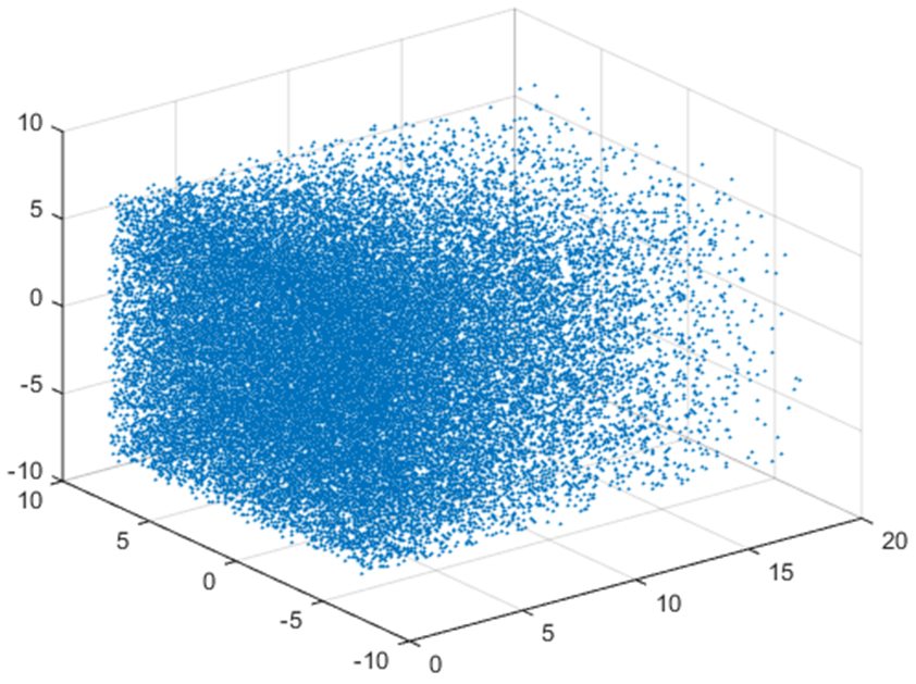
 The estimation of variance could be found in suggested reading. They perfectly match each other. We could also display our result in figure:
變異數的估計我們之前沒有討論,請讀者自行參閱推薦文章。我們發現它們完美契合。我們也可以把實驗結果印成圖:
 The tiny blue dots are the recorded particles. Noted that our slime mold only record a little particles compared to the number of particles in the background. It's really amazing, isn't it? And that's all about our this series, gradient sensing. I hope you enjoy it.
藍色的點是被黏菌偵測到的粒子,注意到我們的黏菌只記錄了一點點粒子而已,就得到了很正確的估計,這是不是很神奇呢?可見maximum likelihood的威力。 我們這個系列就到這邊結束囉,希望各位會喜歡。
所以我們來比較一下理論的數值和黏菌估計出來的背景梯度:
cz_theoretical = -(1/(width_source*width_source))/(2*D);
cz_best_estimate = mean(cz_estimated);
var_cz_theoretical = -cz_theoretical*x_Boundary/(12*pi*D*r_Dicty^3*tMeasure);
var_cz_estimate = var(cz_estimated);
display(cz_theoretical);
display(cz_best_estimate);
display(var_cz_theoretical);
display(var_cz_estimate);
toc;
And the result we get:
然後實際run出來的結果長這樣:

變異數的估計我們之前沒有討論,請讀者自行參閱推薦文章。我們發現它們完美契合。我們也可以把實驗結果印成圖:
%% plot result
[x,y,z] = sphere;
figure
surf(r_Dicty*x+location_Dicty(1),r_Dicty*y+location_Dicty(2),r_Dicty*z+location_Dicty(3));
hold on;
axis square;
Detected_List(isnan(Detected_List(:,1)),:)=[];
x_particle_all(isnan(x_particle_all(:,1)),:)=[];
if ~isempty(Detected_List)
    scatter3(Detected_List(:,1),Detected_List(:,2),Detected_List(:,3) , 1);
end
scatter3(x_particle_all(:,1),x_particle_all(:,2),x_particle_all(:,3) , 1);
toc;

藍色的點是被黏菌偵測到的粒子,注意到我們的黏菌只記錄了一點點粒子而已,就得到了很正確的估計,這是不是很神奇呢?可見maximum likelihood的威力。 我們這個系列就到這邊結束囉,希望各位會喜歡。
/*---------Divider---------*/
Suggested reading and reference:
推薦閱讀與參考資料:
Endres, R. G. & Wingreen, N. S. (2008). Accuracy of direct gradient sensing by single cells. PNAS 105(41): 15749-15754.
Suggested reading and reference:
推薦閱讀與參考資料:
Endres, R. G. & Wingreen, N. S. (2008). Accuracy of direct gradient sensing by single cells. PNAS 105(41): 15749-15754.
Comments
Post a Comment